Capital Budgeting with Monte Carlo Simulations in Python

Capital budgeting is a necessary exercise that often gets neglected in the analytics domain. While Excel has add-ons for Monte Carlo simulations, running these analyses on Google Sheets or macOS Numbers is nearly impossible. This article demonstrates how to use Python for robust capital budgeting with Monte Carlo simulations.

The Problem

Traditional capital budgeting relies on single-point estimates for cash flows. But real-world variables like costs, revenues, and growth rates are uncertain. A Monte Carlo simulation addresses this by:

Defining probability distributions for each variable
Sampling from these distributions thousands of times
Calculating the outcome (NPV, IRR) for each sample
Analyzing the distribution of results

A Practical Example: Cloud Migration

Consider a common challenge many tech companies face: Should we migrate our on-premise workloads to the cloud?

We need to compare:

Current cash flows for running, maintaining, and expanding on-premise infrastructure
Projected cash flows for cloud migration and ongoing cloud costs

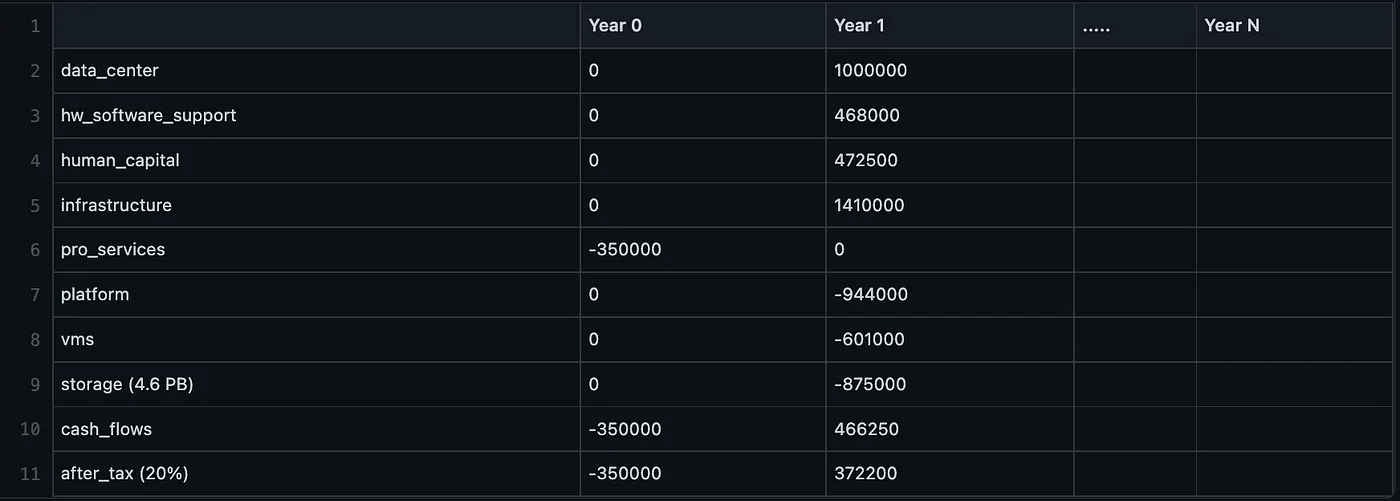Cash flow structure for capital budgeting Figure 1: Cash flow structure for the cloud migration analysis. Each row represents a cost category with Year 0 (initial investment) and projected years. Negative values indicate costs, positive values indicate savings.

Key Financial Metrics

Net Present Value (NPV)

NPV calculates the present value of future cash flows, discounted by a hurdle rate:

 1
 2
 3
 4
 5
 6
 7
 8
 9
10
11
12
13
14
15
def calculate_npv(cash_flows: list, hurdle_rate: float) -> float:
    """
    Calculate Net Present Value of cash flows.

    Args:
        cash_flows: List of cash flows by period (index 0 = period 0)
        hurdle_rate: Discount rate (e.g., 0.10 for 10%)

    Returns:
        Net Present Value
    """
    npv = 0
    for t, cf in enumerate(cash_flows):
        npv += cf / (1 + hurdle_rate) ** t
    return npv

Internal Rate of Return (IRR)

IRR is the discount rate that makes NPV equal to zero—essentially, the return above breakeven:

 1
 2
 3
 4
 5
 6
 7
 8
 9
10
11
12
13
14
15
16
from scipy.optimize import brentq

def calculate_irr(cash_flows: list) -> float:
    """
    Calculate Internal Rate of Return.

    Args:
        cash_flows: List of cash flows (must have sign changes)

    Returns:
        IRR as a decimal
    """
    def npv_at_rate(rate):
        return sum(cf / (1 + rate) ** t for t, cf in enumerate(cash_flows))

    return brentq(npv_at_rate, -0.99, 10.0)

Setting Up the Monte Carlo Simulation

Define Probability Distributions

Each uncertain variable gets a probability distribution based on domain expertise:

 1
 2
 3
 4
 5
 6
 7
 8
 9
10
11
import numpy as np
from scipy import stats

# Define distributions for key variables
distributions = {
    "on_prem_maintenance": stats.norm(loc=500000, scale=50000),
    "cloud_compute_cost": stats.norm(loc=300000, scale=75000),
    "migration_cost": stats.triang(c=0.5, loc=200000, scale=300000),
    "growth_rate": stats.uniform(loc=0.05, scale=0.15),
    "on_prem_expansion": stats.norm(loc=1000000, scale=200000),
}

Run the Simulation

 1
 2
 3
 4
 5
 6
 7
 8
 9
10
11
12
13
14
15
16
17
18
19
20
21
22
23
24
25
26
27
28
29
30
31
32
33
34
35
36
37
38
39
40
41
42
43
44
45
46
47
48
49
50
def run_simulation(n_simulations: int = 10000,
                   periods: int = 5,
                   hurdle_rate: float = 0.10) -> dict:
    """
    Run Monte Carlo simulation for cloud migration decision.

    Returns:
        Dictionary with NPV and IRR distributions
    """
    npv_results = []
    irr_results = []

    for _ in range(n_simulations):
        # Sample from distributions
        on_prem_maint = distributions["on_prem_maintenance"].rvs()
        cloud_cost = distributions["cloud_compute_cost"].rvs()
        migration = distributions["migration_cost"].rvs()
        growth = distributions["growth_rate"].rvs()
        expansion = distributions["on_prem_expansion"].rvs()

        # Calculate cash flows for each period
        cash_flows = [-migration]  # Initial investment

        for year in range(1, periods + 1):
            # Savings = On-prem costs - Cloud costs
            on_prem_total = on_prem_maint * (1 + growth) ** year

            # Add expansion costs every 3 years for on-prem
            if year % 3 == 0:
                on_prem_total += expansion

            cloud_total = cloud_cost * (1 + growth * 0.5) ** year

            savings = on_prem_total - cloud_total
            cash_flows.append(savings)

        # Calculate metrics
        npv = calculate_npv(cash_flows, hurdle_rate)
        npv_results.append(npv)

        try:
            irr = calculate_irr(cash_flows)
            irr_results.append(irr)
        except ValueError:
            pass  # IRR doesn't exist for some scenarios

    return {
        "npv": np.array(npv_results),
        "irr": np.array(irr_results)
    }

Analyze Results

 1
 2
 3
 4
 5
 6
 7
 8
 9
10
11
12
13
14
results = run_simulation(n_simulations=100000)

# Calculate statistics
print(f"NPV Statistics:")
print(f"  Mean: ${results['npv'].mean():,.0f}")
print(f"  Median: ${np.median(results['npv']):,.0f}")
print(f"  Std Dev: ${results['npv'].std():,.0f}")
print(f"  5th Percentile: ${np.percentile(results['npv'], 5):,.0f}")
print(f"  95th Percentile: ${np.percentile(results['npv'], 95):,.0f}")
print(f"  Probability NPV > 0: {(results['npv'] > 0).mean():.1%}")

print(f"\nIRR Statistics:")
print(f"  Mean: {results['irr'].mean():.1%}")
print(f"  Probability IRR > Hurdle Rate: {(results['irr'] > 0.10).mean():.1%}")

Sample Output:

NPV Statistics:
  Mean: $847,234
  Median: $823,156
  Std Dev: $312,456
  5th Percentile: $298,412
  95th Percentile: $1,423,891
  Probability NPV > 0: 94.2%

IRR Statistics:
  Mean: 28.3%
  Probability IRR > Hurdle Rate: 91.7%

This output tells us the cloud migration has a 94.2% probability of positive NPV and a 91.7% chance of exceeding our 10% hurdle rate—a strong investment case.

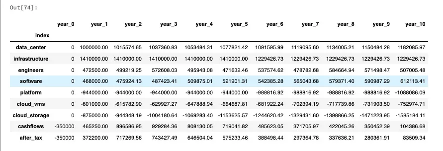10-year cash flow projections from Monte Carlo simulation Figure 2: Complete 10-year cash flow projection from a single Monte Carlo iteration. The bottom rows show cumulative cash flows and after-tax values used to calculate NPV and IRR.

Visualizing the Results

 1
 2
 3
 4
 5
 6
 7
 8
 9
10
11
12
13
14
15
16
17
18
19
20
21
22
23
24
25
26
import matplotlib.pyplot as plt

fig, axes = plt.subplots(1, 2, figsize=(14, 5))

# NPV Distribution
axes[0].hist(results['npv'], bins=50, edgecolor='black', alpha=0.7)
axes[0].axvline(x=0, color='red', linestyle='--', label='Breakeven')
axes[0].axvline(x=results['npv'].mean(), color='green',
                linestyle='--', label=f"Mean: ${results['npv'].mean():,.0f}")
axes[0].set_xlabel('NPV ($)')
axes[0].set_ylabel('Frequency')
axes[0].set_title('NPV Distribution')
axes[0].legend()

# IRR Distribution
axes[1].hist(results['irr'], bins=50, edgecolor='black', alpha=0.7)
axes[1].axvline(x=0.10, color='red', linestyle='--', label='Hurdle Rate (10%)')
axes[1].axvline(x=results['irr'].mean(), color='green',
                linestyle='--', label=f"Mean: {results['irr'].mean():.1%}")
axes[1].set_xlabel('IRR')
axes[1].set_ylabel('Frequency')
axes[1].set_title('IRR Distribution')
axes[1].legend()

plt.tight_layout()
plt.savefig('monte_carlo_results.png', dpi=150)

The resulting histograms show the full distribution of possible outcomes, making it easy to visualize the range of scenarios and communicate risk to stakeholders.

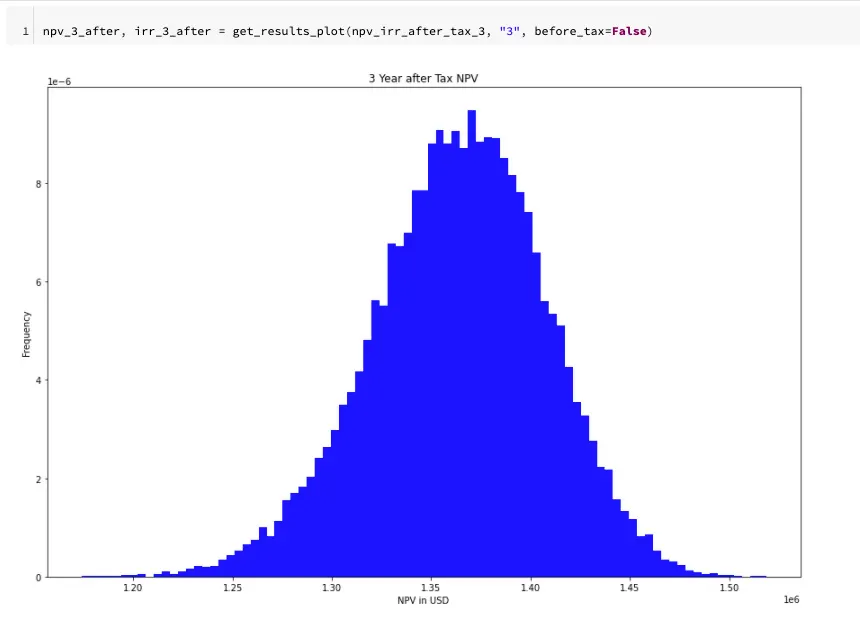3-Year after-tax NPV distribution Figure 3: NPV distribution at the 3-year mark from 100,000 Monte Carlo iterations. The distribution centers around $1.35M with a roughly normal shape, indicating consistent positive returns in the short term.

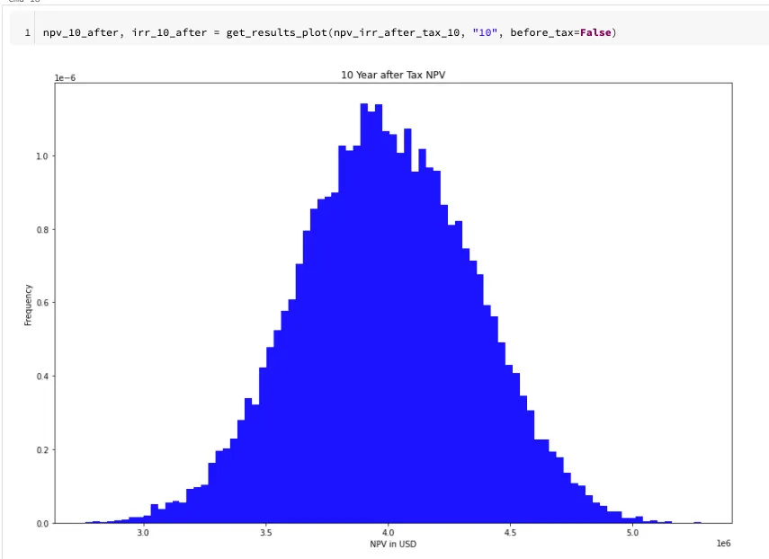10-Year after-tax NPV distribution Figure 4: NPV distribution at the 10-year mark. The mean shifts to approximately $4M, demonstrating how the investment value compounds over time. The wider spread reflects increased uncertainty over longer horizons.

Making the Decision

With Monte Carlo results, you can make informed decisions:

Scenario	Recommendation
P(NPV > 0) > 90%	Strong case for investment
P(NPV > 0) between 50-90%	Proceed with caution, consider risk tolerance
P(NPV > 0) < 50%	Investment likely unfavorable

Additionally, compare the IRR distribution against your hurdle rate to understand the probability of achieving your minimum required return.

Extending the Analysis

This template extends beyond cloud migration. Use it for:

Factory development decisions
Data compression cost savings analysis
New product launch feasibility
Equipment replacement timing
R&D investment evaluation

The complete notebook is available on GitHub.

Conclusion

Monte Carlo simulation transforms capital budgeting from a single-point estimate exercise into a probabilistic analysis. By understanding the full distribution of possible outcomes, you can:

Quantify uncertainty in investment decisions
Communicate risk to stakeholders
Make decisions aligned with your organization’s risk tolerance
Identify which variables have the greatest impact on outcomes

Python provides all the tools needed for sophisticated financial analysis without relying on expensive Excel add-ons or limited spreadsheet capabilities.

Originally published on CodeX