Data Optimization for Compacted Partitions: Achieving 77% Storage Reduction

When managing petabyte-scale data lakes, small non-optimal leaf files within partition directories can severely impact performance and inflate storage costs. At True Digital Group, we developed an intelligent data optimization strategy that achieved 77% storage reduction and 90% runtime improvements across our largest datasets.

The Small File Problem

The core challenge involves files significantly smaller than the HDFS block size (typically 256MB). For large columnar data formats like ORC and Parquet, optimal file sizes should range between 512MB to 1024MB. Spark’s default spark.sql.shuffle.partitions=200 setting often creates suboptimal file distributions, particularly in pipelines that apply business logic transformations introducing shuffles.

Naive Approaches: Coalesce vs. Repartition

Coalesce

Using coalesce() avoids shuffles, making it faster. However, it cannot guarantee equal file distribution across partitions, limiting its optimization potential.

Repartition

Using repartition() introduces shuffles, which enables equally-sized leaf files. The downside is that it may disrupt the natural data ordering that benefits columnar compression, potentially decreasing or even increasing file sizes unpredictably.

Neither approach alone provides optimal results for large-scale data optimization.

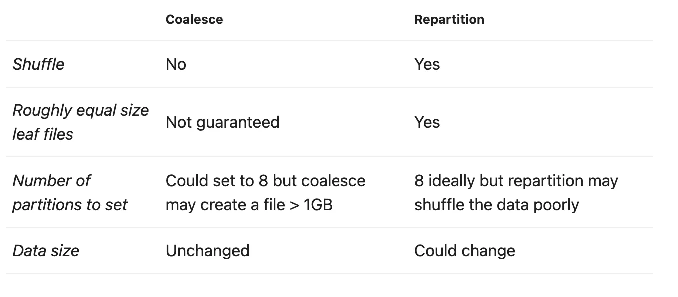Figure 1: Comparison of coalesce vs repartition. Coalesce avoids shuffles but can’t guarantee equal file sizes; repartition enables equal sizes but may change data size unpredictably.

The Optimized Approach: Linear Ordering

The recommended strategy involves ordering data by high-priority columns identified by domain experts and power users. The key guidelines:

• Select no more than 10 columns for ordering
• Prioritize columns frequently used in queries
• Place lowest-cardinality columns first
• Leverage columnar compression benefits through hierarchical ordering

 1
 2
 3
 4
 5
 6
 7
 8
 9
10
11
12
13
14
15

# Option 1: Repartition first, then sort within each partition
df.repartition(target_partitions).sortWithinPartitions(
    "region",
    "customer_segment",
    "product_category",
    "transaction_date"
)

# Option 2: Global sort then coalesce (preserves ordering)
df.orderBy(
    "region",
    "customer_segment",
    "product_category",
    "transaction_date"
).coalesce(target_partitions)

Important: Using orderBy().repartition() would lose the ordering since repartition triggers a shuffle. Use sortWithinPartitions after repartitioning, or coalesce after a global sort to preserve ordering.

Results at True Digital Group

Testing on two weeks of production data demonstrated significant improvements:

Across all optimized datasets, we achieved 2.331 petabytes of cumulative storage savings as of June 2021.

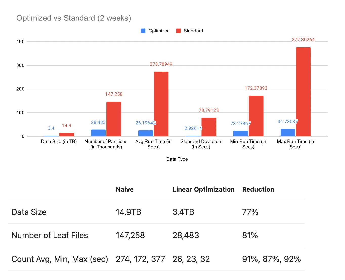Figure 2: Optimized vs standard comparison over 2 weeks of data. Linear ordering achieved 77% data size reduction (14.9TB → 3.4TB), 81% fewer leaf files, and 90%+ runtime improvements.

Figure 3: Monthly partition sizes in production. The consistent ~500GB bars represent already-optimized partitions, while the 2.5-3TB spikes are new incoming data prior to optimization—demonstrating the dramatic size difference.

Financial Impact

Using AWS S3 Singapore pricing, 795TB of savings (accounting for 3-factor replication) yielded approximately $19,287 in monthly cost savings.

Advanced Optimization: Space-Filling Curves

For even greater optimization, space-filling curves (Hilbert, Morton/Z-ordering) map multi-dimensional indices to single dimensions more optimally than linear approaches.

Z-Ordering

Z-ordering uses bit interleaving to create a sort order that considers multiple columns simultaneously. For example, coordinates {(1, 1), (1, 8), (2, 1), (3, 1)} become {(1, 1), (2, 1), (3, 1), (1, 8)} after Z-ordering, allowing secondary columns to influence the final ordering.

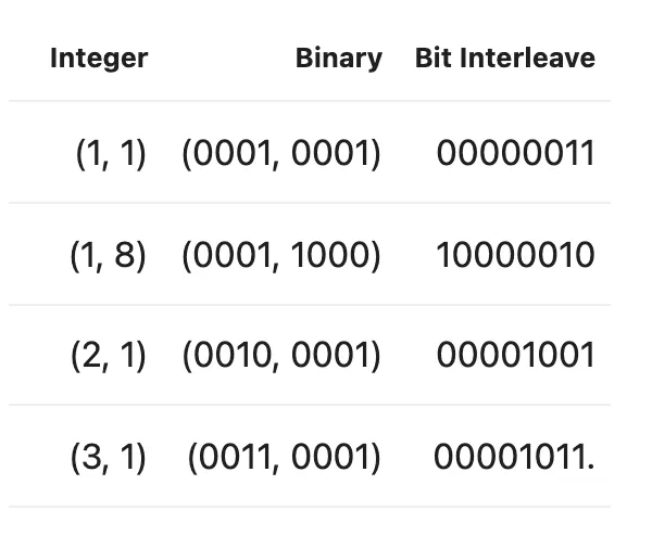Figure 4: Z-ordering bit interleaving. Integer coordinates are converted to binary, then bits are interleaved to create a single sort key that preserves locality across multiple dimensions.

1
2
3
4
5

# Pseudocode for Z-ordering
z_indexed_df = df.withColumn(
    "z_index",
    z_order_udf(col("dim1"), col("dim2"), col("dim3"))
).orderBy("z_index")

Performance Gains

Testing demonstrated an additional 16% improvement over linear ordering when Z-ordering was applied—reducing 1.5TB to 334GB versus 398GB with linear ordering alone.

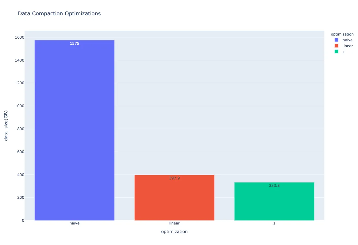Figure 5: Final comparison of optimization approaches. Naive: 1,575GB → Linear ordering: 398GB (75% reduction) → Z-ordering: 334GB (additional 16% improvement).

Validation

Maintaining data integrity throughout the optimization process is critical. We validate using:

1. Count verification: Ensure row counts match before and after optimization
2. Min/Max validation: Verify boundary values remain consistent
3. Checksum comparison: Compare checksums between naive and optimized datasets

Conclusion

Over 18 months of implementation, we achieved 50-70% data savings across our largest datasets. The benefits extended beyond storage:

• Improved cluster utilization
• Reduced server expansion needs
• Faster pipeline execution
• Lower computational resource requirements

The key insight is that intelligent ordering based on actual usage patterns—not just arbitrary repartitioning—unlocks columnar format compression potential that naive approaches miss.

Originally published on Towards Data Science